fastKDE and xarray
This notebook demonstrates basic usage of fastkde.plot with xarray.
import numpy as np

try:
    import fastkde
    import xarray
except:
    # install fastkde
    !pip install --upgrade fastkde
    import fastkde

import matplotlib.pyplot as plt
For this example, we will generate data with the following relationships:
\[x := \mathcal{N}(0,\pi)\]
\[y := \mathcal{N}(\sin(x), 1)\]
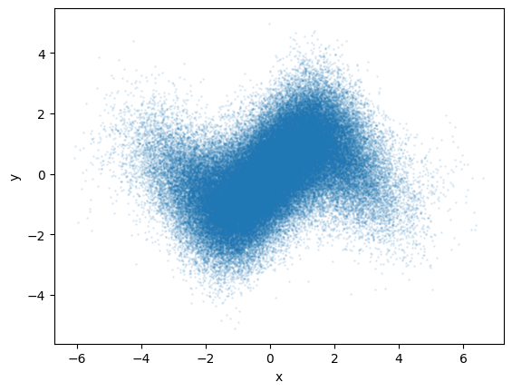
""" Sample the two variables """
N = int(1e5)
x = np.random.normal(size=N, scale=np.pi / 2)
y = np.sin(x) + np.random.normal(scale=1, size=N)

# plot the data
plt.scatter(x, y, s=1, alpha=0.1)
plt.xlabel("x")
plt.ylabel("y")
plt.show()
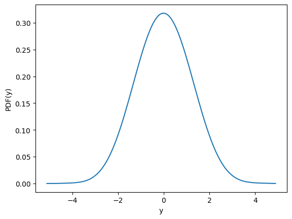
""" Calculate and plot 1D PDFs. """

# calculate the PDFs of x and y
pdf_x = fastkde.pdf(x, var_names=["x"])
pdf_y = fastkde.pdf(y, var_names=["y"])

# plot PDF(x)
pdf_x.plot()
plt.show()

# plot PDF(y)
pdf_y.plot()
plt.show()

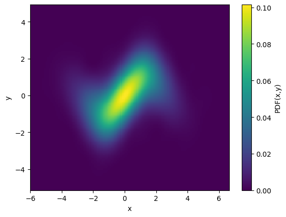
""" Compute the 2D PDF. """

pdf = fastkde.pdf(x, y, var_names=["x", "y"])
pdf
<xarray.DataArray (y: 128, x: 128)> Size: 131kB
array([[0., 0., 0., ..., 0., 0., 0.],
       [0., 0., 0., ..., 0., 0., 0.],
       [0., 0., 0., ..., 0., 0., 0.],
       ...,
       [0., 0., 0., ..., 0., 0., 0.],
       [0., 0., 0., ..., 0., 0., 0.],
       [0., 0., 0., ..., 0., 0., 0.]], shape=(128, 128))
Coordinates:
  * x        (x) float64 1kB -5.971 -5.872 -5.773 -5.674 ... 6.418 6.517 6.617
  * y        (y) float64 1kB -5.107 -5.029 -4.95 -4.871 ... 4.732 4.811 4.89
Attributes:
long_name: PDF(x,y)""" Plot the PDF using xarray. """
# plot the 2D pdf
pdf.plot();
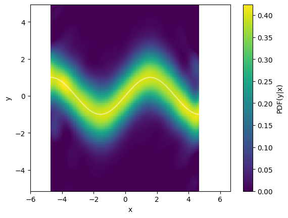
""" Compute and plot the conditional PDF using xarray. """

cpdf = fastkde.conditional(y, x, var_names=["x", "y"])

# plot the conditional
cpdf.plot()

# plot the true conditional mean
plt.plot(cpdf.x, np.sin(cpdf.x), color="white", alpha=0.5);